
Backtesting Mean-Variance Alternatives
A practical comparison of mean-variance alternatives across a diversified ETF universe

In a previous post, I discussed several alternatives to mean-variance optimization (MVO), which are summarized below:
In this post, I’m going to put them all to the (back)test. To keep things simple but also practical, I’ll use a common universe of ETFs representing different asset classes and regions, and I’ll make some choices about how to group them into buckets to avoid undue concentrations.
Asset Universe and Data
I start with the following universe of ETFs. Although there are arguably some better (i.e. cheaper) ETFs for at least some of the asset classes, I chose these to maximize the length of the backtest period.
The ETFs belong to different asset classes/regions To allow me to control overall exposures, I assign them to an upper level “allocation bucket”. I would note that both my definitions of asset class and allocations buckets involve a degree of subjectivity. For example, I could have put REITs, Commodities, and Gold into one big bucket and called it “Alternatives”, but I preferred to split real estate from commodities and gold.
The ETFs all have different inception dates. To extend the backtest as much as possible, I first download total return series for the ETFs as well as their corresponding indices from Bloomberg. Then, for each ETF, if the ETF data starts after the index data, I backfill the series using the index returns. This gives me synthetic series starting in 2000 for almost all ETFs, the exceptions being VNQI (start date: 02/01/2001) and BNDX (start date: 04/01/2013).
After completing this step, I end up with the following series:
Setting Up the Backtest
I use 3 years of daily data to estimate inputs for all methods, so the backtests start in 2003. On each rebalance date, I require an ETF to have available data over the last 3 years. Portfolios are rebalanced at the end of each month, and held for one month.
To avoid extreme allocations to individual assets/buckets, I constrain the optimizer for most optimizations to avoid solutions that drift too far from a diversified multi-asset allocation. At the allocation bucket level, I use the following constraints:
At the individual ETF level, I use the following constraints:
In my view, these constraints embed a relative flexible asset allocation policy, while also preventing overly concentrated portfolios.
I used simple historical estimates for expected returns and Ledoit-Wolf shrinkage estimator for the covariance matrix.1 All optimizations were done using the skfolio python package. I clean-up weights to remove very small weights, and use some reasonable failsafes in case optimizations fails.
The Models
I consider the following allocation models. With the exception of the risk budget portfolio, all other optimizations are done using the constraints discussed previously. Also, it should be noted that both the Global 60/40 Benchmark and the 1/N portfolio are feasible under the set of constraints.
1. Global 60/40 Benchmark:
A simple strategic allocation: 40% U.S. equities, 20% international equities, and 40% bonds, with a global tilt through EFA, EEM, and BNDX. The allocations within equity (SPY, EFA, EEM) and fixed income (AGG, BNDX) represent loosely the breakdown of the market cap of the markets represented by the ETFs.2
2. 1/N Portfolio
This is an equally weighted portfolio of all available assets on each month. Note that applying 1/N across these ETFs/asset classes is not an innocuous or view-free allocation decision. It implies the following allocations: 33.33% to equity, 22.2% to bonds, 22.22% to REITs, and 22.22% to Commodities/Gold (11.11% each).
3. Minimum Variance Portfolio (MVP)
This portfolio chooses weights to minimize overall portfolio volatility available within the constraints.
4. Mean-Variance Optimization with Target Volatility (MVO σ=10%)
This portfolio chooses the highest-return it can find while targeting a fixed volatility level of 10%.
5. Mean-Semivariance Portfolio (Mean-SV)
This portfolio optimizes expected return subject to a target semivariance equal to the realized semi-variance of the Global 60/40 portfolio. The semi-variance is calculated relative to a target return of zero.
6. Mean-CVaR Portfolio (Mean-CVaR)
This portfolio optimizes with respect to tail risk rather than volatility. CVaR measures the average loss in the worst part of the return distribution, so this approach is designed to be more sensitive to extreme downside events. I use a confidence level β=0.95 and a target CVaR equal to the CVaR of the Global 60/40 portfolio.
7. Maximum Diversification Portfolio (MDP)
This portfolio maximizes the diversification ratio, favoring assets that contribute distinct risk exposures rather than moving closely together.
8. Risk Budget Portfolio (RB)
This portfolio allocates portfolio risk, rather than capital, across assets. Note that the risk budget approach is sensitive to the choice of the assets. For this reason, I decided to implement risk budgets across the allocation buckets:
Equities: 40% (split equally between SPY, EFA, and EEM)
Fixed Income: 40% (split equally between AGG and BNDX)
Real Estate: 10% (split equally between IYR and VNQI)
Commodities/Gold: 10% (split equally between DBC and GLD)
This results in ETF-level risk budgets that vary between 5% to 20%. Note that a risk parity solution at the ETF level would allocate 11.1% (1/9) to each ETF, which would result in a different risk budget at the bucket level.3 It should also be noted that for the RB portfolio, the asset-level and bucket constraints on portfolio weights do not apply.
Results
The backtests cover the period from February 2003 to April 2026. The table below shows summary statistics of all the models.
Before looking at the numbers, it’s important to note a few things:
Since the strategies have different levels of risk, comparison of most statistics is not appropriate. In special, comparing returns and maximum drawdowns would be misleading.
The alternative allocation models I considered have different objectives. Some of the metrics are directly related to certain objectives; others are not. For example, none of the methods directly relate to maximum drawdown. While we can certainly analyze the realized maximum drawdowns, we can’t really make any conclusions about the methods in general based on this.
In the case of the risk-based models (MVP, MDP, and RB) in particular, it’s important in my view to look at statistics related to what these methods try to achieve. For example, within the methods that implement the constraints, MVP achieves the lowest volatility, which suggests the objective of this model is attained.4 Likewise, when looking at MDP, we should probably look at other metrics that directly relate to the diversification ratio. For RB, the primary objective is to attain the desired risk budget, which the method does.
In order to make the strategies easier to compare, the table below shows the same statistics, but with the volatility of all strategies scaled to 10%. The best performing strategies in terms of risk-adjusted ratio metrics (Sharpe and Sortino ratio) are the mean-risk optimizations, which all produce very similar results.
The animation below shows the equity curves for all vol-scaled strategies.
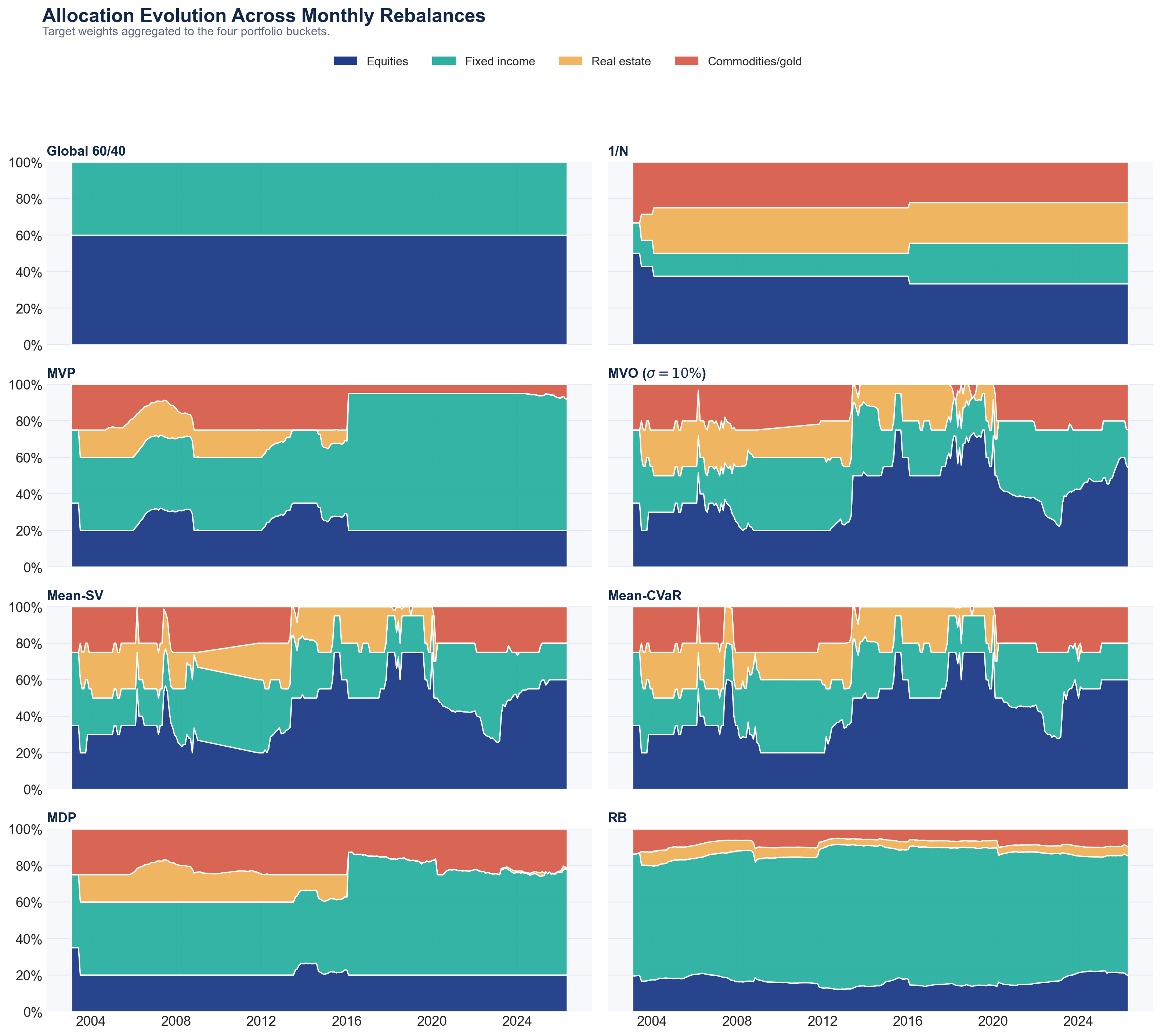
The graphs below show the allocations on each rebalance date. A few points to note:
MVP allocates significantly to bonds, as expected. Over the second half of the sample, the bucket level constraint is binding most of the time.
The mean-risk (MVO, Mean-SV, Mean-CVaR) allocations follow almost identical patterns, with more volatility in allocations over time compared with MDP and RB.
MVP and MDP do not allocate to REITs at all over the second half of the sample. This is explained by the fact that the correlation between REITs and equity is significantly higher over the second period. As a result, there is little diversification to be gained by adding REITs to the portfolio.
The allocations of RB are very bond-heavy (as expected) and generally stable over time.
The table below shows the average monthly turnover of the models, computed from drifted weights and assuming a conservative one-way transaction cost of 25bps.5 Mean-risk approaches have higher turnover compared to other strategies, but the transaction costs remain very manageable.
Final Thoughts
The objective of this post was to show a practical implementation of alternative methods to mean-variance optimization (MVO) for a diversified asset universe covering major asset classes. In this backtest, alternative mean-risk portfolio construction approaches, such as mean-semivariance and mean-CVaR, produced almost identical results to MVO. After scaling the strategies to the same volatility, the mean-risk optimization models also delivered better risk-adjusted performance than simpler allocations, including a global 60/40 benchmark and the 1/N allocation, as well as other risk-based approaches, such as risk budget and maximum diversification.
Once embbeded inside a sensible asset-allocation policy, mean-risk optimizations, including MVO, worked well.
I started this post with no prior expectation for how MVO would perform relative to the other methods. In fact, I have no horse in this race, and I believe we should follow the empirical evidence. Despite being often criticized, MVO performed well in this application, even though I relied on simple historical estimates of expected returns and imposed only relatively simple constraints. Of course, this does not mean that MVO is appropriate in every situation, or that more sophisticated methods cannot deliver better solutions, particularly if investors have specific preferences about risk and return.
One important caveat is that the mean-risk optimizations use historical expected returns. In a nine-asset universe with strong long-run differences across realized asset-class returns, this can make a lot of difference. The result should therefore not be interpreted as evidence that historical mean returns are generally reliable forecasts. Rather, it shows that in this particular universe, sample period, and constrained implementation, mean-risk optimization was able to exploit return differences without producing pathological portfolios.
With 3 years of daily data per asset and only 9 assets, the sample covariance matrix would have worked just as well.
On the periods prior to BNDX availability, the strategy allocates 40% to AGG.
The risk budget in this case would be as below. I don’t like this allocation as it gives over 40% of the total risk budget to Commodities and Gold.
Equities: 33.3%
Fixed Income: 22.2%
Real Estate: 22.2%
Commodities/Gold: 22.2%
The fact that RB produces lower volatility than MVP is explained by the fact that the RB portfolio is not subject to the same constraints. Since fixed income has lower risk, RB allocates more to this bucket to balance the risk contributions.
I estimate transaction costs as follows (example for MVO σ=10%):