
Pockets of Replicability (Post #3)
A series of short articles on finance research replicability. On this issue: a surprisingly heated debate about Bayesian model comparison in asset pricing.

In their 2018 JF paper, Comparing Asset Pricing Models, Barillas and Shanken (BS) proposed a Bayesian asset pricing test to help sort through the so-called “factor zoo”, the collection of hundreds of asset pricing factors “discovered” over the last 30 years or so. his widely cited paper was part of a broader revival of interest in Bayesian methods in asset pricing, and the multifactor model they identified as having the largest posterior probability was used in several papers as an alternative to common benchmarks like the Fama and French 3- and 5-factor models, or the models proposed by Hou, Xue, and Zhang.
The main idea of the BS approach was to use an improper Jeffreys prior for the beta coefficients and the residual covariance matrix:
while keeping an informative prior for alphas conditional on other parameters:
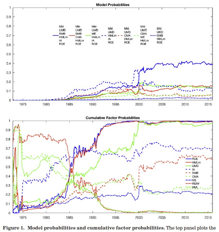
where k is chosen based on plausible values for the maximum Sharpe ratio. Under these choices, they obtained a closed form way of calculating posterior model and factor probabilities, which allows for model comparisons. Using a set of 13 candidate asset pricing factors, they compute posterior model probabilities recursively over time. The graph below suggests that the model in blue, which includes six factors (market, momentum, size, monthly updated value, investment, and ROE), seems to dominate others.
The Problem
In 2020, Chib, Zeng and Zhao (CZZ) published (also on JF) the aptly called paper “On Comparing Asset Pricing Models”, in which they showed that BS’s calculations do not lead to correct posterior model probabilities. CZZ state (emphasis mine):
In this paper, we revisit the framework of Barillas and Shanken (2018), BS henceforth, and show that the Bayesian marginal likelihood-based model comparison method in that paper is unsound. Hence, the BS “marginal likelihoods” each depend on an arbitrary constant, which voids the ranking of models by the size of the marginal likelihoods and invalidates any conclusions drawn from such a method about the underlying data-generating process (DGP).
The issue arises because the prior for the betas is improper (i.e., not a valid probability distribution that integrates to 1). Because of that, multiplying this improper prior by any positive value produces the same improper prior, which in turn implies that the marginal likelihoods (loosely speaking, the probability of the data given the model) are determined only up to a constant. If all models shared the same prior, this constant would cancel out in model comparisons.1 However, as CZZ show, this is not the case in the BS framework. The key requirement for valid Bayesian model comparison is that the priors across competing models must be induced from a common underlying measure so that any arbitrary constants cancel in Bayes factors. CZZ show that this coherence condition fails in the BS setup, and then go on to propose a prior under which these conditions hold, and thus model comparison is valid.
How much difference does it make? Using simulations, CZZ show that under different DGPs and sample sizes, the BS prior never identifies the correct null model, in the sense that the highest posterior probability model under the BS prior is never the true model. This is disputed to some degree by BS.
The BS Riposte
Not surprisingly, Barillas and Shanken disputed this critique and responded in a follow-up paper. In a reply to CZZ called “Comparing Priors for Comparing Asset Pricing Models”, BS state that the approach described in CZZ had been discussed in communications between BS and CZZ, in response to an earlier version of CZZ’s paper. CZZ note in their paper that the issue had been raised by a reader of an earlier draft. As it turns out, one of authors in BS had been a reviewer of the earlier version of CZZ’s paper.
BS also argue that the measure used by CZZ to compare the results under the two different priors was overly simplistic, as it relied on a binary outcome (assigning higher posterior probability to the correct model). In addition, they argue that CZZ pre-selected statistically significant models, which may induce some bias.
Applied CZZ
In “Winners from Winners: A Tale of Risk Factors”, Chib, Zhao, and Zhou (let’s call them CZZ2) put the CZZ prior to an empirical test using two sets of factors:
A smaller list of 12 “benchmark” factors for which there’s some support in the literature (Fama and French factors, Hou, Xue, and Zhang factors etc).
A larger list of 125 additional factors from the factor zoo (from Hou et al., 2020).
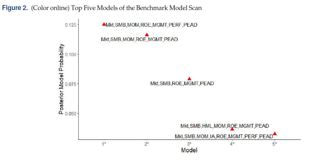
They first run a benchmark scan using the initial set of benchmark factors, which supports a 7-factor model:
Next, they use this 7-factor model to first rule out factors from the larger set (with 125 factors).2 This approach reduces the model space by keeping only 24 “true anomalies” relative to the 7-factor model. Note that the model space is still huge: with a total of 36 factors (12 benchmark plus 24 true anomalies), the total number of models is over 68 million. To further reduce dimensionality, they use the first 12 principal components (PCs) of the 24 anomalies, reducing the model space to “only” about 17 million models. The resulting models with highest posterior probability all include the PCs of the anomalies. In addition, the best model from this extended model scan outperforms the best model from the original scan over the 12 benchmark factors.
Other Bayesian Approaches for the Factor Zoo
I wrote a paper with Soosung Hwang in which we applied a Bayesian variable selection methodology to investigate the selection of asset pricing factors using individual stocks. Using individual stocks has the advantage of bypassing certain issues that can arise from grouping stocks into portfolios. We used a hirerarchical model with indicator variables γj that are equal to 1 if a factor is included in the model, and 0 otherwise. Since we did not use improper priors, the issues described previously do not affect model comparison. One of the advantages of the specific hierarchical setup we used is that it is possible to integrate out the models parameters and obtain the posterior distribution of the vector γ directly through MCMC simulation, which then can be used to obtain the posterior factor and model probabilities. Our results suggested that:
of the 88 factors we considered, only a few appeared to be relevant;
of these, only the market and size factors coincide with the factors from widely used factor models, like the Fama-French 5-factor model or the Hou et al q-factor model;
many different factor combinations have similar posterior probability, suggesting that model uncertainty is pervasive and that the search for a single factor model is unlikely to give a definitive answer in asset pricing.
Bryzgalova et al. (2023) proposed a Bayesian approach to compare different linear asset pricing models by focusing directly on estimation of the stochastic discount factor (SDF). Although they use improper priors, they are careful to only use them for nuisance parameters, such that their effect is canceled out in Bayes factors calculations. In addition to identifying high-posterior probability factors that should be included in any SDF, a key empirical result from their paper is that the SDF is dense in the space of observable factors. In other words, due to substantial model uncertainty, aggregation through Bayesian model averaging outperforms sparse representations. This is similar to what we found in our paper, and in line with the findings on Giannone, Lenza, and Primiceri (2021), that dense models outperform sparse ones in various applications in economics and finance.
Final Thoughts
The use of Bayesian methods in asset pricing research has several advantages. The Bayesian approach is flexible, handles high dimensionality well, and naturally provides answers when model uncertainty is pervasive. However, as this short discussion shows, there are some pitfalls in Bayesian model comparison. Improper priors are often harmless for parameter estimation, but they can be problematic for model comparison because Bayes factors depend on the normalization of the prior.
An Oversimplified Example
To illustrate the issue with improper priors, consider a simple example. Suppose we observe data:
where σ2 is know, and want to compare
against
Under the alternative model, suppose we use the improper flat prior:
for some arbitrary constant C.
The marginal likelihood under M0 is a function only of the data. Let’s denote it by m0(x).
The marginal likelihood under the alternative is defined only up to an arbitrary positive constant, because the prior is improper. When we integrate the likelihood with respect to this prior to compute the marginal likelihood, this constant carries through the calculation.The marginal likelihood under the alternative then becomes
where A(x) depends only on the data. The Bayes factor comparing the two models is
where B(x)=A(x)/m0(x). Since C can be chosen arbitrarily, the Bayes factor, and therefore the posterior model probabilities, are not uniquely defined.
At the end of this post, I include an oversimplified example of the problem of Bayesian model comparison with improper priors.
For each of the 125 factors, they run a Bayesian comparison of two models, one with the intercept, and one without the intercept. If the Bayes factor favors the model with the intercept, they concluded that that factor is a true anomaly, and include it in the next step.