
Portfolio Optimization: What Could Go Wrong?
A lot, actually...

Mean-variance optimization is one of those ideas that is both foundational and strangely easy to caricature. In theory, it gives us the cleanest possible answer to a portfolio choice problem. In practice, small changes in the inputs can lead to large changes in the portfolio. This post is about the second part. I’ll show some concrete examples of how easily things can go wrong when portfolio optimization is implemented naïvely, and how some of these issues can be attenuated in practice. I’ll focus only on mean-variance optimization (MVO), the most vanilla of all portfolio optimization approaches.
Python code for all the examples shown in this article is provided at the end.
The Mean-Variance Optimization Problem
Given n assets, we are trying to build an efficient portfolio in a mean-variance sense. For a target level of expected return µ, we want the portfolio with the lowest risk possible.1
Any finance textbook gives us the following recipe:
Find the minimum variance portfolio (MVP) and compute its expected return. The MVP is the solution of the problem above without the target expected return constraint.
Create a grid from the expected return of the MVP to a maximum expected return.
Solve the problem above for each target expected return, store portfolio weights, expected returns, and standard deviations.
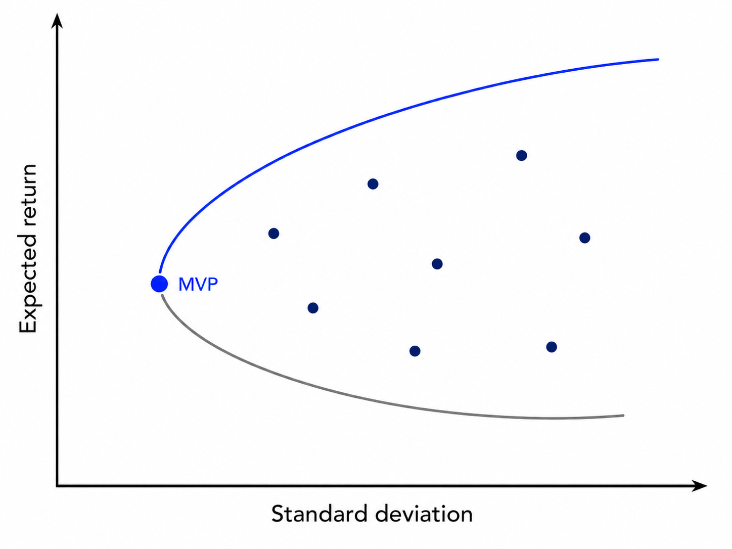
Plot the resulting set of portfolios in standard deviation-expected return space.
The result is the so-called efficient frontier, i.e., the set of portfolios with the lowest risk for each level of expected return (or alternatively, with highest expected return for each level of risk). This is the starting point for many classic results in finance which I’m not going to discuss here.
Problems with MVO
Already we can identify some potential issues:
We don’t really know the expected returns of the assets or their covariance matrix;
We’re assuming that the investor’s preference is fully captured by expected returns and the covariance matrix of returns;
Everything is static (this is a single period model);
The framework doesn’t take into account practical considerations, such as transaction costs.
I will come back to some of these issues in a future article. For now, let’s focus on the first one. Since we do not know the expected returns and covariances, the best we can do is to estimate them, which brings estimation error into the problem. The standard Markowitz machinery is not designed to take that into account. A common critique is that MVO is an “error maximizer”, but this is a critique of the estimation process, not of the method.
This distinction matters. Optimization does not create information. It operates on whatever information is in the inputs. If the inputs contain signal, optimization can turn small edges into meaningful portfolio gains. If the inputs contain mostly noise, optimization can amplify that noise into concentrated bets.
Among the inputs to be estimated, there is a pecking order in terms of the impact on the resulting portfolios:
Expected returns→Variances→Covariances
The intuition is simple: expected returns enter the optimizer as the reward for taking risk, so small differences in estimated means can dominate the allocation. Variances determine the scale of risk for each asset, while covariances determine diversification benefits across pairs.
The estimation of expected returns is the most critical. Not only are expected returns difficult to estimate precisely, but small differences in expected return estimates can significantly affect the resulting portfolios. In terms of the covariance matrix, errors in the variances are approximately twice as important as errors in the covariances.2 There are also known issues in estimating covariances, especially in high dimensions (hundreds or thousands of assets), but there are many methods that can attenuate these issues.
Many empirical studies that find lackluster performance for MVO portfolios estimate inputs directly from historical returns. Interestingly, this is clearly at odds with what Markowitz himself suggested. His 1952 paper opens with the following statement:
The process of selecting a portfolio may be divided into two stages. The first stage starts with observation and experience and ends with beliefs about the future performances of available securities. The second stage starts with the relevant beliefs about future performances and ends with the choice of portfolio. This paper is concerned with the second stage…
To use the E-V rule in the selection of securities, we must have procedures for finding reasonable μi and σij. These procedures, I believe, should combine statistical techniques and the judgment of practical men.
So dismissing MVO because naïve implementations based on historical return estimates perform poorly feels a bit like throwing the baby out with the bathwater. That is, the fact that estimates based only on past returns produce poor results should not automatically disqualify the optimization process.
One interesting aspect regarding the estimation of expected returns is that even a small forecasting edge can significantly improve results. Expected return estimates based only on realized returns are mostly noise, but firm characteristics and other variables can be used to construct forecasting models with low, but nonzero, predictive power. This is a point I will come back to in a future article.
Practical Examples
The rest of this post is concerned with simple illustrations of the very real issues that arise when MVO is applied using naïve estimates from historical returns. These examples are pedagogical but typical of what happens in practice if we implement MVO “out of the box”. Examples 1 through 4 illustrate common problems that arise in naïve MVO implementations. Examples 5 and 6 show simple ways to attenuate some of them.
Example 1: Input sensitivity
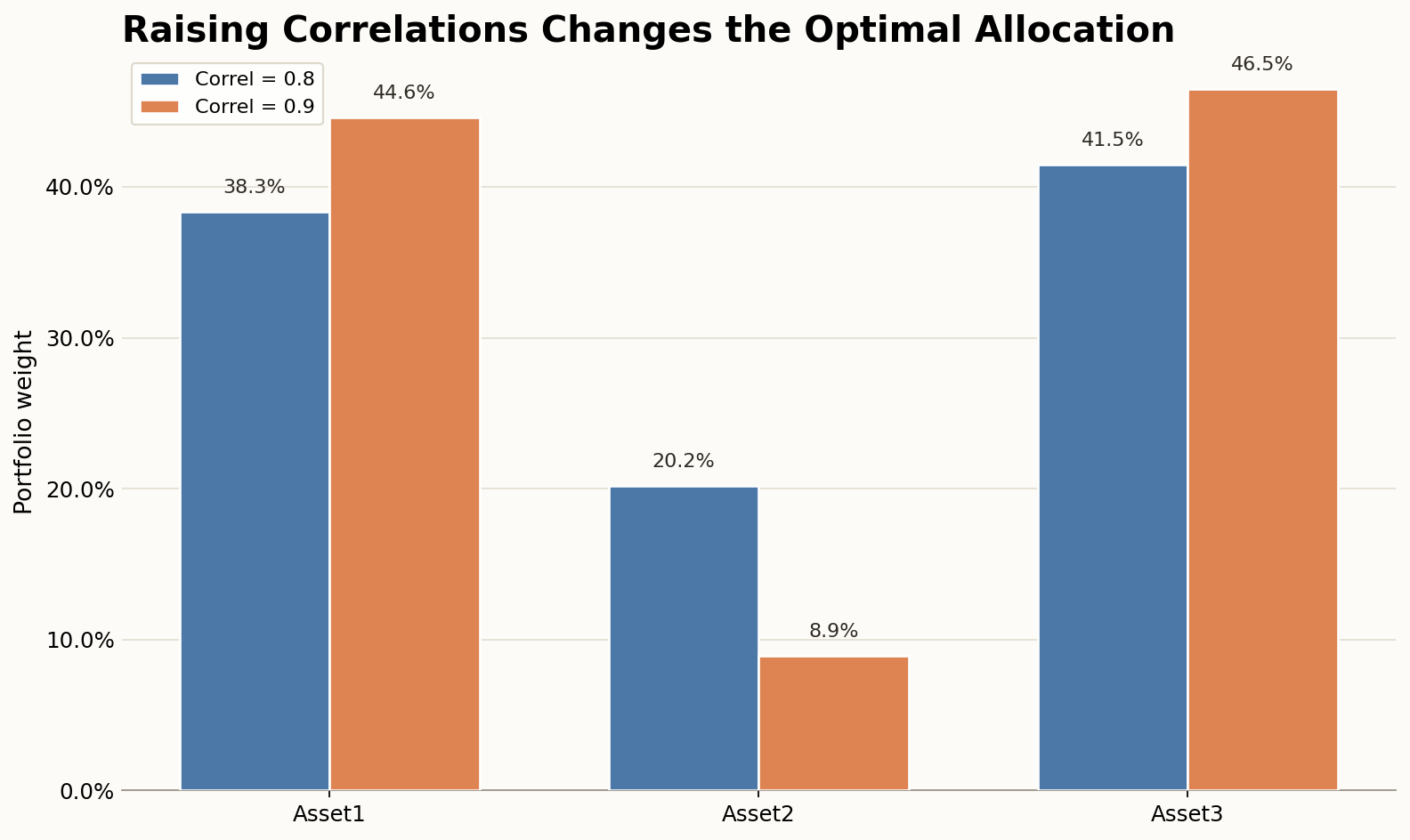
A common issue with MVO is the sensitivity of the results to changes in the inputs. Consider the example below. There are three assets with the characteristics below. Assume all correlations are equal to 0.8, and the objective of the manager is to maximize the expected return for a 15% volatility target.3
If we solve the problem, we get the following portfolio weights:
Now suppose we increase all pairwise correlations from 0.8 to 0.9. In this case, we get the following solution:
An apparently small change in the correlation leads to large differences in portfolio weights.
Example 2: Estimation Error
Example 1 illustrated the fact that MVO weights are very sensitive to the inputs. We also know that financial returns are very noisy, and the inputs are estimated under significant estimation error, especially expected returns. But that doesn’t mean that we can take covariance matrix estimates for granted. Even with a small number of assets, sample variability can have an important impact.
In this example, we consider an extremely simple application of MVO. There are only two assets:
SPY (U.S. equities)
TLT (Long-Term U.S. Treasuries)
And we are estimating the minimum variance portfolio (MVP) of the two assets on a given date. In the two-asset case, the MVP is calculated in closed form as
Therefore, we only need to estimate 3 parameters:
The variance of SPY
The variance of TLT
The covariance between SPY and TLT
Suppose we decide to estimate these parameters using 5 years of daily returns for the two ETFs. This means we have approximately 1,260 daily return observations for each asset, which is a relatively generous sample for estimating only three parameters.
Using 5 years of daily data ending in March 2026, we get the following estimates:
SPY volatility: 17%
TLT volatility: 16%
Correlation (SPY,TLT): 0.0712
The corresponding MVP allocates 46% to SPY and 54% to TLT, resulting in a volatility of 12%. The reduction in risk is due to the low correlation.
In this simple example with only 3 parameters to estimate, how much sampling variability exists? That is, if we had used a slightly different sample, we would have obtained different estimates. To quantify the variability in these estimates, we use a technique known as bootstrapping. The idea is to construct new samples by randomly drawing, with replacement, from the original sample. The graphs below were generated with 1,000 bootstrap samples.
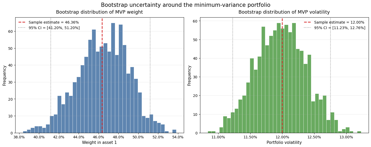
As we can see, even in this simple case in which data is relatively abundant, there’s a substantial amount of uncertainty. A 95% confidence interval for the MVP weight on SPY is [41.20%, 51.20%], while the corresponding interval for MVP volatility is [11.23%, 12.76%].
Example 3: Corner Solutions/Extreme Concentration
Another common issue in naïvely implemented MVO portfolios, especially when weights are left unconstrained, is the emergence of corner solutions. The optimizer finds a solution that invests almost all capital in just a small subset of the assets, leading to extreme portfolio concentration.
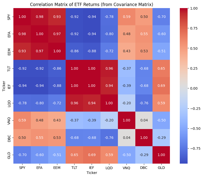
Let's consider the problem of optimizing a portfolio using the following ETFs representing different asset classes:
U.S. Stocks (SPY)
International Stocks (EFA)
Emerging Stocks (EEM)
Long-Term U.S. Treasuries (TLT)
Intermediate-Term U.S. Treasuries (IEF)
U.S. Corporate bonds (LQD)
Real Estate (VNQ)
Commodities (DBC)
Gold (GLD)
The objective is to find the portfolio with the highest expected return subject to a target volatility of 10%.
Below are solutions obtained from a naïve implementation of MVO on a specific date (December 2019). Expected returns and the covariance matrix estimates are obtained using sample moments from the previous 3 years of daily data. The “Unconstrained” solution allows short positions, while the “Long-Only” requires non-negative weights. In both cases, the full investment constraint (sum of weights = 1) is used.
The unconstrained solution invests in all ETFs, but the level of leverage is unreasonable (gross leverage of over 600%). The optimizer takes large opposite positions in IEF and LQD. The two ETFs are highly correlated (ρ=0.94), but have a difference in expected returns, so the optimizer aggressively buys LQD (expected return 6.7%) and shorts IEF (expected return 4%). While the positions are extreme, this is not unexpected. In the absence of other constraints, the optimizer is trying to take advantage of the fact that the two assets seem like close substitutes but have a return differential.
The long-only solution, on the other hand, is extremely concentrated. It invests only in SPY (78.7%) and GLD (21.3%).
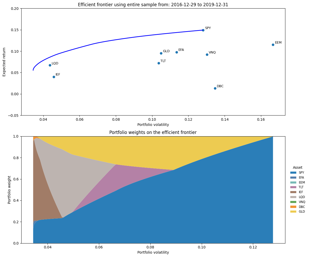
What about other efficient portfolios? The graph below shows the entire efficient frontier under the long-only constraint (wi ≥ 0). As we can see below, the entire frontier lacks diversification, investing on average in only 3 assets at any given level of volatility.
Example 4: Instability of Optimal Weights
Considering the same setup of Example 3, let’s explore how the optimal weights for the target volatility of 10% in the long-only case evolve if we rebalance the portfolio at each month end. As can be seen in the graph below, the optimal allocations can vary dramatically over time. In Example 3, the optimal allocations as of December 2019 were concentrated in SPY (~80%) and GLD (~20%). But we can see that, prior to that date, the GLD allocation was replaced by either TLT or LQD.
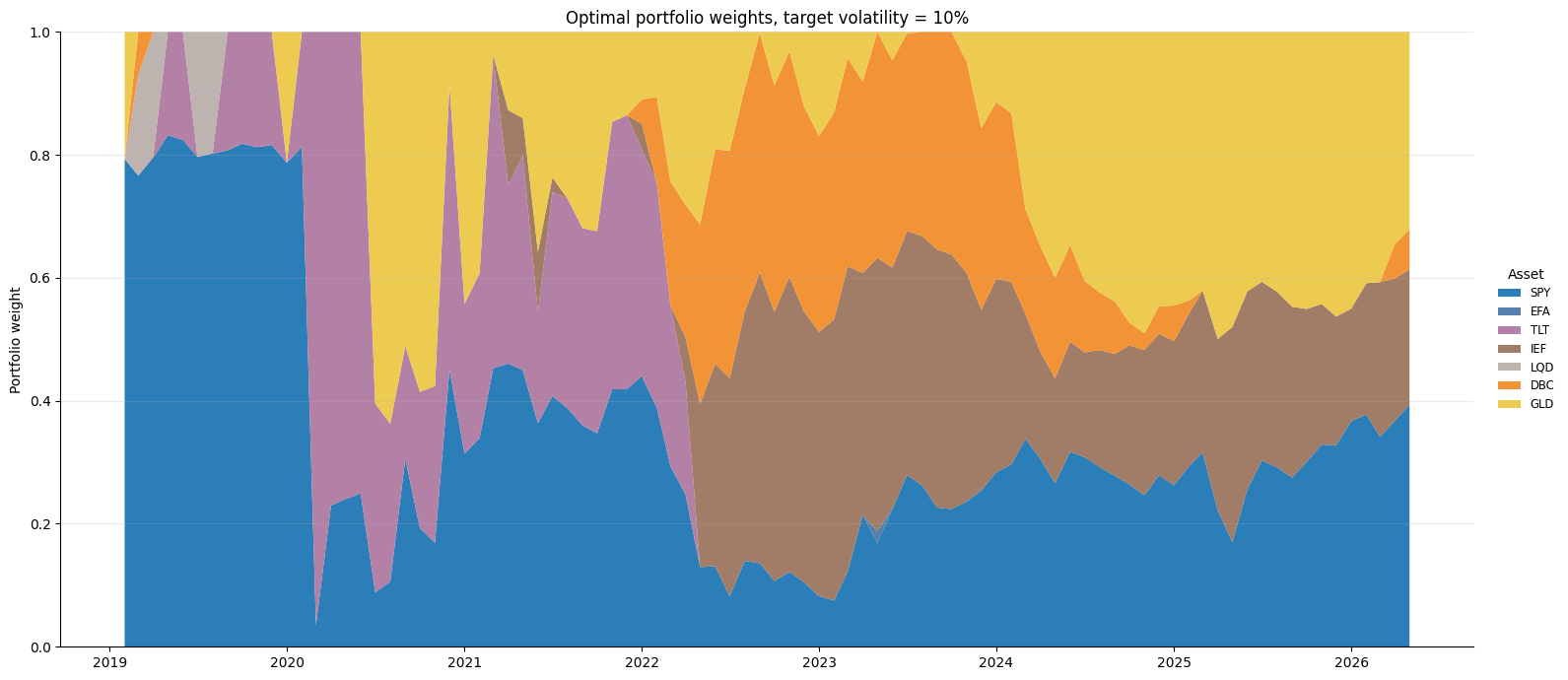
The COVID shock shifts allocations dramatically due to changes in the estimated parameters. As shown below, the optimal portfolio moves to an almost 20% allocation to TLT in January 2020, and then abruptly allocates almost 100% to TLT in February 2020.
Once again, this is not unexpected. We relied on sample moments for the optimization. When the sample moments abruptly changed, the optimization results changed accordingly. This is not necessarily bad: it would make sense to reduce exposure to risky assets during this period. But without forward-looking estimates, the best the optimizer can do is react when the sample moments change. Using shorter samples will lead to faster reactions, with higher portfolio turnover.
Another interesting question is the extent to which empirical regularities can make their way into the optimization process. For example, using past returns to construct estimates of expected returns can introduce a momentum effect in the portfolio construction process. This illustrates an important nuance: using historical returns as expected returns is not always an accidental mistake. Sometimes it is an intentional signal design choice. The problem is that once expected returns are estimated from recent returns, the optimizer needs additional discipline, usually in the form of constraints.
JPMorgan designed an index based exactly on this idea. The JP Morgan Efficiente 5 index uses a set of 12 ETFs and constructs an optimal portfolio using mean-variance optimization with a lookback window of 6 months to estimate expected returns. The idea behind the short lookback period is to try to capture time series momentum in the ETFs. To get around the lack of diversification we have seen in this example, they impose maximum weights per ETF and per asset class. The inclusion of these additional constraints is the simplest approach to attempt to discipline MVO results, as I’ll illustrate in the next example.
Example 5: Adding Constraints
One of the most commonly used approaches to deal with the concentration issues in MVO is to introduce constraints on the portfolio weights. We explore the impact of simple constraints for the long-only optimal portfolio in Examples 3 and 4. We consider the following portfolios:
Long-only: the same portfolio in Example 3 (positive weights with full investment constraint).
Max. asset weight: long-only portfolio with an additional constraint that the weight on any asset is capped at 20%.
Max. asset class weight: long-only portfolio with the constraint that the weight on any asset is capped at 20% and additional caps per asset class.
For the last one, we divide portfolios into 3 asset classes for simplicity as follows:
Equity: SPY, EFA, EEM. The upper bound for the combined weights is 50%.
Fixed Income: TLT, IEF, LQD. The upper bound for the combined weights is 50%.
Alternatives: VNQ, GLD, DBC. The upper bound for the combined weights is 30%.
For each case, we obtain the optimal portfolio with a target volatility of 10% at the end of December 2019. The solutions in each case are shown below. The first column shows the same overly concentrated portfolio from Example 3, which invests in only two out of the nine assets. The introduction of the maximum weight constraint at the asset level (column “Max. asset weight”) forces the optimizer to diversify. The constraint is binding for SPY and GLD, but the portfolio now invests in six assets. Finally, the introduction of the additional asset class constraints (column “Max. asset class weight”) improves diversification a bit more, although two assets (TLT and VNQ) are still left out.
As we can see, introducing constraints into the portfolio optimization process has the practical effect of improving diversification. There are also theoretical reasons for why adding constraints can be beneficial, as they induce a shrinkage effect on the covariance matrix, which attenuates estimation error.
Example 6: A Simple Resampling Approach
In Example 2, I used bootstrapping to assess the variability in MVP weights. An interesting approach that can be used to mitigate several of the issues with MVO illustrated above is to apply resampling to the portfolio optimization process. A typical process works as follows:
Estimate expected returns and covariance matrix from the original sample.
Generate many simulated or bootstrap samples.
For each sample, estimate a new µ and Σ.
Compute an efficient frontier for each resample.
Average the portfolio weights across resamples at corresponding points on the frontier.
Evaluate the averaged portfolios using the original estimates.
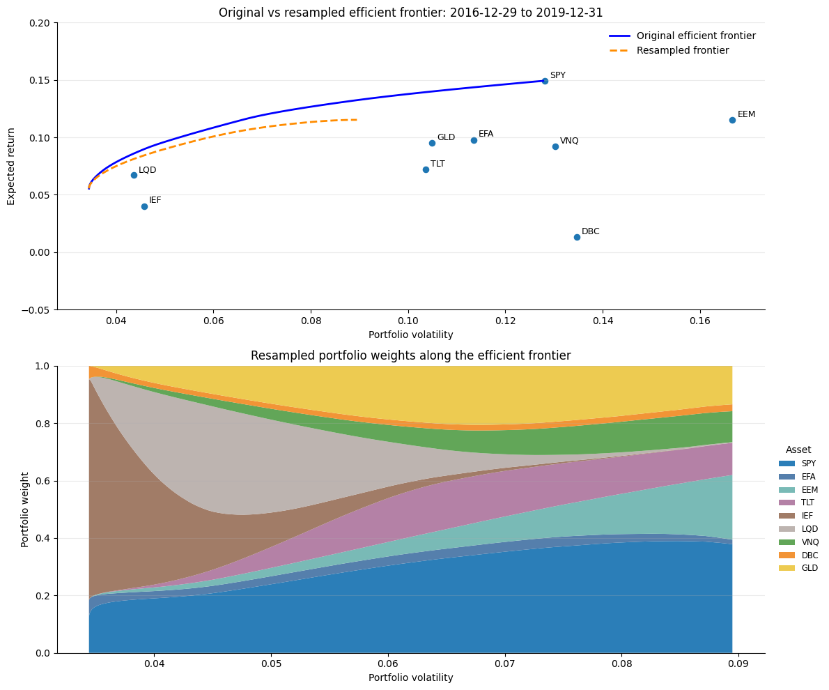
I apply this approach to the multi-asset-class portfolio of the 9 ETFs on December 2019 (for comparison with the results in Examples 3-5). The resampling step uses 500 bootstrap samples.
The resampled frontier is shorter and plots below the full sample one (top chart). The bottom chart shows that the resampling approach improves diversification significantly. In particular, all assets are now part of the frontier, and the concentrations are much less extreme. Note that the resampled frontier below does not include any constraints, either at the individual asset or the asset class level. Nevertheless, the allocations are much less extreme compared to a single optimization.
The resampled frontier is much more diversified because it averages the optimal weights obtained from many slightly different versions of the data. In the original sample, mean-variance optimization tends to put large weights on the assets that look best in-sample, especially those with high estimated returns, low estimated risk, or favorable estimated correlations.
But these estimates are noisy, so the identity of the “best” assets changes across bootstrap samples. An asset that receives a large weight in one resample may receive a smaller weight, or no weight, in another. When the weights are averaged across many resampled frontiers, these unstable extreme positions are diluted, while assets that are consistently useful across samples retain higher weights. The result is a smoother and more diversified allocation that sacrifices some in-sample efficiency in exchange for lower sensitivity to estimation error.
Final Thoughts
Mean-variance optimization (MVO) is often criticized as yielding nonsensical or impractical results. This article shows practical examples that illustrate:
how sensitive MVO solutions can be to small changes in inputs;
how MVO can produce overly concentrated portfolios or extreme long-short positions;
how naïve sample-moment estimates can lead to unstable allocations over time;
how constraints and resampling can reduce, though not eliminate, these problems.
MVO is not the only game in town. Other portfolio construction approaches are designed, at least in part, to handle some of the issues illustrated in this article:
The Black-Littermann model starts from the idea that market weights contain useful equilibrium information, then allows investors to incorporate views with an explicit degree of confidence.
Bayesian approaches, more generally, model uncertainty about expected returns, covariances, or other inputs directly rather than treating estimates as known.
The Total Portfolio Approach uses the strategic asset allocation process to define a fund’s return objective and overall risk budget, but treats the resulting benchmark as a guide rather than a binding allocation. It recognizes the uncertainty in long-term forecasts and gives investment teams more discretion to deploy risk across the total portfolio as opportunities and market conditions change.
Risk parity reduces reliance on expected return estimates by focusing instead on how much each asset contributes to total portfolio risk.
Parametric portfolio policies allow investors to link portfolio weights directly to asset characteristics that may contain information about expected returns.
While there are many alternative portfolio construction methodologies, I would argue that MVO remains useful because it makes the trade-off between return, risk, and diversification explicit. Knowing its practical limitations, and ways to avoid them, remains essential.
Python Code
Notebooks that replicate all examples in this article are provided below for supporters of the Systematically Biased.
Keep reading with a 7-day free trial
Subscribe to Systematically Biased to keep reading this post and get 7 days of free access to the full post archives.