A Deep Dive Into Risk Parity

Allocating risk, not capital: a practical guide to risk parity, risk budgeting, and hierarchical allocation

This post is divided into two parts. The first part introduces the basic intuition behind risk parity and provides an example in the two-asset case. The second part, which is exclusive for paid subscribers, goes deeper into the mechanics of risk budgeting, risk measures, factor risk parity, hierarchical risk parity, and long/short applications, and the recent literature.

In previous posts, I explored alternatives to mean-variance optimization and showed the results of a backtest for a universe of ETFs representing different asset classes. I touched briefly on risk parity in these posts.

On this post, I’ll explore risk parity in more detail and discuss some of the more recent research on the topic.

---

What is Risk Parity?

Risk parity is an investment management approach that focuses on the allocation of risk, rather than capital. Traditional approaches, such as mean-variance optimization, take as inputs estimates of expected returns of the assets as well as their covariances, and produce as output a capital allocation to achieve a certain objective (e.g., maximizing expected return for a given level of risk). Risk parity asks a different question: what capital allocation produces equal risk contributions from each asset?

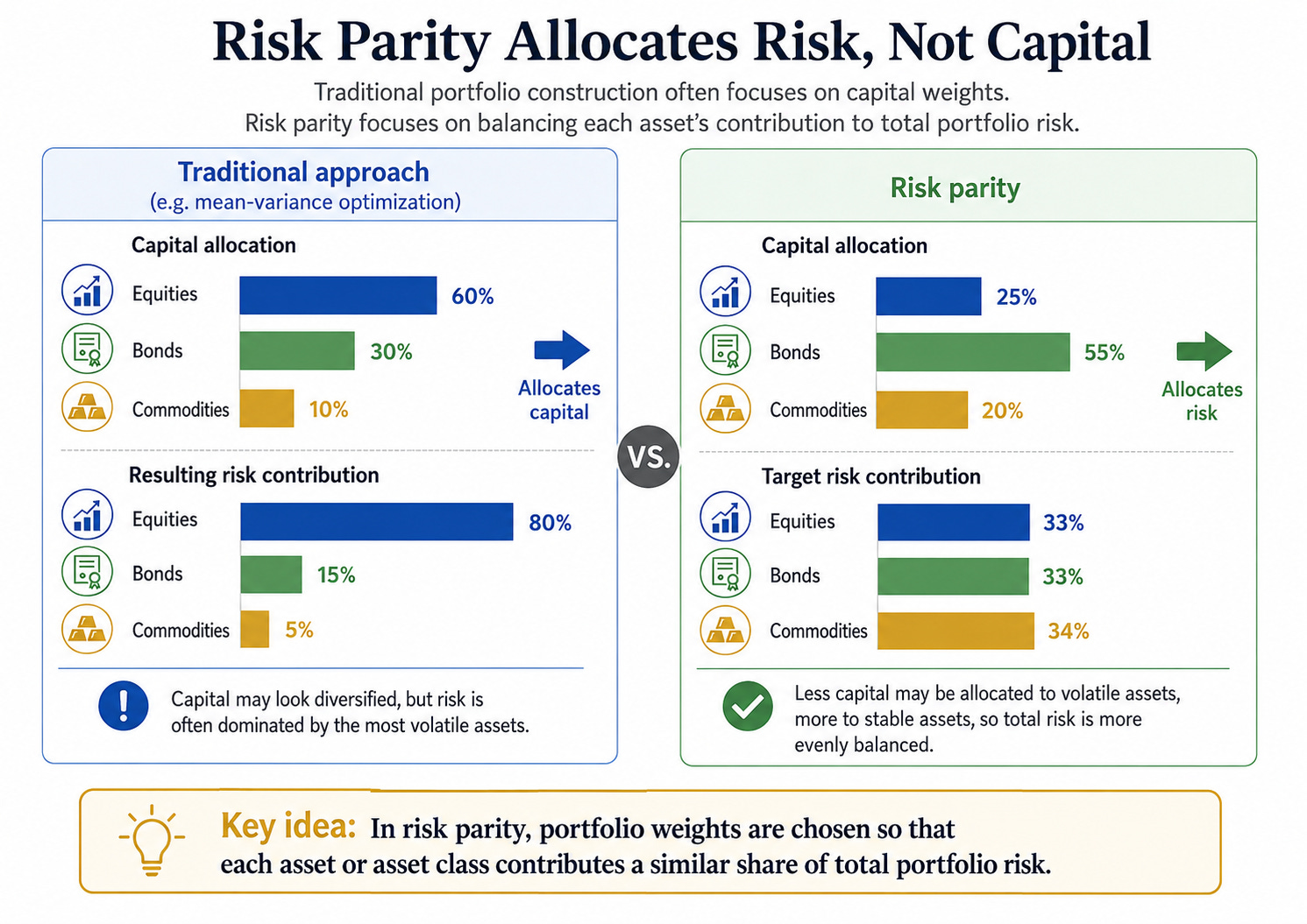
Risk parity is a relatively new approach to investment management. The idea dates back to the 1990s, with the first product¹ being launched in 1996, and the term “risk parity” only being coined in the 2005 paper by Edward Qian. Other names that are often used interchangeably include “risk budgeting” and “equal risk contributions”. Among these, risk budgeting is the most general one, the idea being that the investor can choose the proportion of total risk allocated to each asset. The risk parity, or equal risk contribution portfolio, corresponds to a special case of the risk budgeting approach, in which all assets receive equal risk allocations.

Risk parity is widely used by institutional investors, both as a tool to build multi-asset class portfolios with balanced risk contributions, to balance risk contributions from different assets in specific trading strategies, such as trend following, or to balance the contribution from multiple trading strategies. It is difficult to know how much capital is managed using risk parity principles. A reasonable reading of published estimates is that dedicated risk parity strategies manage on the order of several hundred billion dollars of capital, with levered economic exposure potentially several times larger.

---

Inverse Vol: a Naive Risk Parity Strategy

A precursor to risk parity is the idea of weighting assets inversely to their volatilities. A typical justification for following such an approach is the fact that the risk of a 60/40 stock/bond portfolio is dominated by the stock component. The inverse-vol approach naturally increases the weights of safer assets, resulting in a more balanced portfolio. An issue that arises with the inverse-vol approach is that the volatility of this portfolio may be too low. In this case, leverage can be used to reach a desired target volatility. Asness et al. (2012) investigated this in the context of a 60/40 stock/bond portfolio over a long sample, showing favorable results for the levered inverse-vol portfolio relative to the market portfolio. The authors argue that leverage aversion could explain why this may happen in practice: since many investors are not allowed (or choose not) to use leverage, the higher return may represent a strategic advantage accruing to the investors who choose to do so.

The inverse vol approach is widely used in trend following programs. For example, in their classic paper on time series momentum, Moskowitz et al. (2012) define the return on a trend following portfolio of S different futures contracts as:

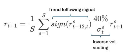
The expression looks complicated, but it is essentially a simple average of S returns on futures contracts, where the return on each contract is multiplied by the sign of the past 12-month return and scaled according to an inverse volatility ratio. The 40% on the numerator is an arbitrary volatility level, justified by the authors to achieve a desired target level of 12% for the realized portfolio volatility. Note that this is calibrated empirically, as it depends on the trend following signals, the volatility estimates, and the diversification, which is not modeled.

The inverse vol approach has the advantage of being straightforward to use, only requiring estimates of the volatilities of the assets. However, because it does not model covariation between assets, in general, it does not produce equal risk contributions across assets or asset classes. This can be achieved with “true” risk parity approaches, at the cost of higher complexity.

---

A Simple Example with Two Assets

A simple way to understand the intuition behind risk parity is to work through a simple portfolio with only two risky assets, using the volatility as a risk measure. In this simple case, there is a closed formula for the risk parity portfolio, and all the calculations can be done by hand. Denote by x=(x_{1 ,} x₂)’ the vector of portfolio weights. The volatility of the portfolio is then

\(\sigma(x)=\sqrt{x_1^2 \sigma_1^2+x_2^2\sigma_2^2+2x_1x_2\rho\sigma_{1}\sigma_2}\)

The risk contribution of an asset i is defined as:

\(RC_i=x_i \frac{\partial \sigma(x)}{\partial x_i}\)

The derivatives in this expression can be calculated using the chain rule:

\(\frac{\partial \sigma(x)}{\partial x_1}=\frac{2x_1\sigma_1^2+2x_2\rho\sigma_{1}\sigma_2}{2\sigma(x)}=\frac{x_1\sigma_1^2+x_2\rho\sigma_{1}\sigma_2}{\sigma(x)}\)

and

\(\frac{\partial \sigma(x)}{\partial x_2}=\frac{2x_2\sigma_2^2+2x_1\rho\sigma_{1}\sigma_2}{2\sigma(x)}=\frac{x_2\sigma_2^2+x_1\rho\sigma_{1}\sigma_2}{\sigma(x)}\)

The risk contributions, therefore, are given by:

\(RC_1=x_1 \frac{\partial \sigma(x)}{\partial x_1}=\frac{x_1^2\sigma_1^2+x_1x_2\rho\sigma_{1}\sigma_2}{\sigma(x)}\)

\(RC_2=x_2 \frac{\partial \sigma(x)}{\partial x_2}=\frac{x_2^2\sigma_2^2+x_1x_2\sigma_{12}}{\sigma(x)}\)

Note that the total portfolio volatility is the sum of the risk contributions:

\(RC_1+RC_2=\frac{x_1^2\sigma_1^2+2 x_1x_2\rho\sigma_{1}\sigma_2+x_2^2\sigma_2^2}{\sigma(x)}=\frac{\sigma^2(x)}{\sigma(x)}=\sigma(x)\)

Suppose that we assume that the portfolio is fully invested, such that x₁+x₂=1. To simplify even more the notation, let’s denote by x the weight in asset 1 and by (1-x) the weight in asset 2. In this case, we can write the risk contributions as:

\(RC_1=\frac{x^2\sigma_1^2+x(1-x))\rho\sigma_{1}\sigma_2}{\sigma(x)}\)

\(RC_2=\frac{(1-x)^2\sigma_2^2+x(1-x)\rho\sigma_{1}\sigma_2}{\sigma(x)}\)

If we require equal risk contributions, we need to solve the equation RC₁=RC₂, which gives the solution:

\(x=\frac{\sigma_2}{\sigma_1+\sigma_2}\)

Notice that:

• the solution does not depend on the correlation between the assets. This is not the case in general, even in the two-asset case.

• the weight on asset 1 is the ratio of the volatility asset 2 to the sum of the volatilities. If asset 1 has higher volatility than asset two, its capital allocation will be reduced.

• this solution is the same one we would get with an inverse vol approach. If we define initial weights x₁=1/σ₁ and x₂=1/σ₂, and then rescale the weights so that they sum to 1, we get:

  \(x_1^*=\frac{\frac{1}{\sigma_1}}{\frac{1}{\sigma_1}+\frac{1}{\sigma_2}}=\frac{\sigma_2}{\sigma_1+\sigma_2}\)

  and similarly for asset 2. So risk parity with two assets, using the volatility as the risk measure, is equivalent to inverse volatility weighting. This is not true in general.

We can now reproduce the results from the stock/bond example in previous post. Stock (SPY) had a volatility of 17.94%, while bond (BND) had a volatility of 5.53%. The risk parity portfolio weight on SPY is then

\(x_{SPY}=\frac{\sigma_{BND}}{\sigma_{SPY}+\sigma_{BND}}=\frac{0.0553}{0.1794+0.0553}=0.2356\)

And the weight on BND is

\(x_{BND}=1-x_{SPY}=0.7644\)

The correlation between SPY and BND had been estimated at 0.1433. Plugging the numbers into the formula for the volatility, we get a volatility of 6.39% for the risk parity portfolio. We can also verify that this portfolio has equal risk contributions (RC₁=RC₂) and that the total portfolio volatility is equal to the sum of the risk contributions.

The risk contribution formulas can be used to compute the risk contributions for any allocation. For example, a 60% SPY/40% BND portfolio in this example has a total volatility of 11.29%, but the risk contributions are very unbalanced, with approximately 93.5% of the total risk coming from the equity allocation, and the remaining 6.5% coming from the bond allocation. This is illustrated in the animation below, in which I plot allocations (left bar) versus risk contributions (right bar).

---

A More General Risk Budget Approach