Beyond Mean-Variance Optimization

Seven ways investors can avoid forecasts, redefine risk, or diversify differently

May 25, 2026

Obs: this post contains some formulas that don’t display properly on mobile. They do display correctly on desktop.

In a previous post, I discussed mean-variance optimization (MVO), and some of the many things that can go wrong when MVO is implemented naively. A big issue with MVO or indeed any portfolio optimization method is estimation error. The animation below shows how unstable the MVO can be when we resample the data.

One of the tricks commonly used in practice to stabilize MVO solutions is the use of constraints, which is related to regularization or shrinkage. Jagannathan and Ma (2003) showed that adding long-only constraints to the optimization problem is equivalent to using a modified covariance matrix, with the effect of shrinking the largest elements of the covariance matrix. If large covariances are due to estimation error, this helps because the shrunk covariance matrix becomes more precise.

There are other ways to achieve this shrinkage, notably by using a more structured estimator for the covariance matrix (e.g. an index model), or by explicitly shrinking the sample covariance estimator towards such a structured target. In cases where enough data are available, or if the optimization problem is already constrained, as in many practical cases, the choice of covariance estimator is much less critical.1

This post is going to look at some alternatives to MVO. The papers mentioned in the post are shown in the references section at the end, and most have presentation decks in the Systematically Biased Library.

But before we dive into the alternatives, let’s take two steps back to consider:

The measure of risk used in MVO.
Some misconceptions about MVO that regularly pop up.

Risk ≠ Variance

Textbook MVO equates risk with variance. One formulation of MVO is in terms of maximizing the mean-variance criterion:

$\max_{w}{\underbrace{w'\mu}_{\text{expected return}} -\frac{1}{2}\gamma \underbrace{w'\Sigma w}_{\text{variance}}} \quad \text{s.t.} \quad w' \mathbf{1}=1$

where γ is a risk aversion parameter. This formulation says that investor utility increases with the portfolio expected return and decreases with its variance.2

However, variance as a measure of risk has shortcomings:

Variance penalizes large positive returns as much as large negative returns.
Variance measures deviations from the mean, which may not be the appropriate level of return targeted by the investor.

Regarding the first point, most investors are not worried about large positive returns. What really matters is downside risk: the occurrence of large, negative returns. Therefore, if returns are not symmetrically distributed, using the variance may not be an appropriate way to measure risk.

The second issue is more subtle. Variance is a statistical measure of dispersion, and the first moment (the expected value) is a natural reference point. However, when it comes to investments or measuring risk, there’s no a priori reason why we should measure deviations relative to the expected return. The investor may have a different benchmark level of return (say, the risk-free rate of return, or a fixed level of return like 5%).

In sum, if returns are not symmetrically distributed about the mean, or if the benchmark level of return is not the mean, variance does not in general coincide with downside risk.

One possibility, in this case, is to use another risk measure. A natural candidate is to replace variance with semivariance, which measures deviations only below a benchmark level of return B, and likewise replace covariances with semicovariances. In fact, Markowitz (1959) had already recognized that semivariance is a more plausible measure of risk than the variance.

Semivariance is not the only option. Another commonly used approach is to use a tail risk measure, such as the conditional Value at Risk (CVaR). We discuss both mean-semivariance and mean-CVaR approaches later on.

Before turning to alternatives, it is worth clearing up two misconceptions that repeatedly appear whenever MVO is discussed.

Myths about MVO

It’s important to remember that the estimation error issues discussed above are not specific to MVO. As a general rule, using noisy inputs (either for µ or Σ) can lead to poor results in any optimization problem, especially if it’s unconstrained. But MVO is often the target of these criticisms, even when the results being discussed have been obtained in a naive setting (µ estimated from historical returns; no or unreasonable constraints).

But there are other persistent myths about MVO, and I recommend the article by Benveniste, Kolm, and Ritter (2024) for a discussion of those. I’ll focus here on two of those myths that are probably the most persistent. The first one is that MVO requires assuming normally distributed asset returns. The second one is that it requires assuming investors have a quadratic utility function. I think one of the reasons that these myths persist is that these assumptions indeed imply mean-variance preferences. However, they are not needed for MVO to be a reasonable approach. Let’s take a quick look at each.

Normally Distributed Returns

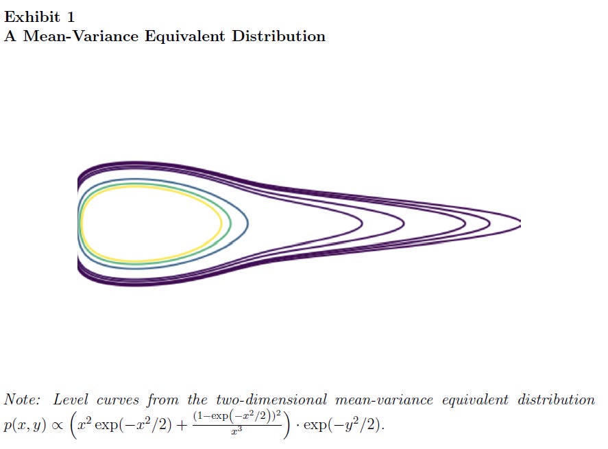
I don’t think that discussing the unreasonableness of assuming normally distributed asset returns is necessary. But if asset returns were normally distributed, then the entire return distribution would be characterized by its mean and variance. Any expected-utility comparison among normally distributed portfolios would therefore reduce to a comparison involving those two moments. While assuming normally distributed returns gives you mean-variance preferences, it is not needed. What matters is the maximization of expected utility. Benveniste, Kolm, and Ritter (2024) define a class of mean-variance equivalent distributions, which have the property that the expected utility maximization for any standard utility function coincides with the maximum of an equivalent MVO problem. Many distributions, including heavy tailed distributions, elliptical distributions, and even some skewed distributions, are mean-variance equivalent.

Example of a mean-variance equivalent distribution from Benveniste, Kolm, and Ritter (2024)

Quadratic Utility

Quadratic utility indeed implies mean-variance preferences, but it also has some economically unreasonable properties. The most relevant is that quadratic utility implies increasing absolute risk aversion. This means that investors would invest less in risky assets as their wealth increases, i.e. risky assets are inferior goods.

As with the normality assumption, quadratic utility implies mean-variance preferences, but is not necessary for MVO to be a reasonable solution to a portfolio allocation problem. Indeed, the mean-variance criterion stated above is not a utility function, but rather an approximation of the expected utility. Under a second-order approximation to expected utility, expected return enters positively and variance enters negatively, with the coefficient on variance governed by risk aversion.3

The rest of this post is going to discuss some alternatives to MVO.

Alternative #0: Keep it Simple (SAA)

The simplest alternative, which existed long before Markowitz proposed MVO, is not to optimize at all. Investors can simply define an asset allocation policy that makes sense in the long run and rebalance their portfolios periodically to maintain it. Of course, defining these allocations requires some assumptions about the expected return and risk of the assets, as well as the investor’s risk preferences.

This kind of approach is sometimes referred to as strategic asset allocation (SAA). The widely used 60/40 benchmark (60% in equities, 40% in bonds) is a canonical example. Many investment products implement variations of this, including options that change the allocations to reduce the portfolio risk at a target date (e.g. for retirement).

Many different SAAs have been proposed, using different assets and asset classes. I implemented several of them in my AssetAllocation package for R (as well as several tactical asset allocation strategies).

Alternative #1: Keep it Simple (the 1/N rule)

Another rule, which is a special case of Alternative #0 and has been extensively studied, is the “Talmudic” or “1/N” rule of allocating equally across investments. This simple rule has the benefits of not requiring forecasts, mechanically enforcing diversification, and keeping turnover low.4 However, 1/N is not assumption-free. The main active decision is shifted from the weights to the definition of the opportunity set.

In terms of empirical performance, there is some controversy. A widely cited study by DeMiguel, Garlappi, and Uppal (2009) ran an out-of-sample horse-race between the 1/N portfolio and 14 mean-variance models across seven datasets, concluding that none of the models outperformed 1/N. Their conclusion: any potential gains due to optimal diversification are more than offset by estimation error.

These results, however, have been questioned by some studies on two fronts:

Kritzman, Page, and Turkington (2010) argue that the outperformance of the 1/N in DeMiguel, Garlappi, and Uppal (2009) is the result of using short samples. When estimates are constructed using longer samples, or simple but reasonable assumptions, Kritzman et al find that optimized portfolios outperform 1/N out of sample.
Allen, Lizieri, and Satchell (2019) make the point that, if investors have even modest forecasting ability, they can benefit substantially from MVO, which they substantiate analytically, via simulation, and empirically through out-of-sample comparisons.

The 1/N rule allocates equally across investments. It requires no forecasts and mechanically forces diversification. Whether 1/N outperforms portfolios obtained using optimization models is debatable.

An example of an investment product based on the 1/N rule is the RSP ETF, which has about $87 billion in assets.

Alternative #2: Minimum Variance Portfolios

The minimum variance portfolio (MVP) is the only portfolio on the mean-variance efficient frontier that doesn’t require estimation of expected returns. It is simply the solution of the problem below: 5

$\min_{w_1,\dots,w_n}{w'\Sigma w} \quad \text{s.t.} \quad \sum_{i=1}^n{w_i}=1$

Because expected returns are harder to estimate and forecast, they are a major source of estimation error in MVO or indeed of any other optimization approach that requires them as inputs. In addition, variances and covariances are more persistent, and therefore more predictable. Therefore, although in principle other portfolios on the efficient frontier may be preferable, the MVP is likely to be estimated with more precision than other efficient portfolios.

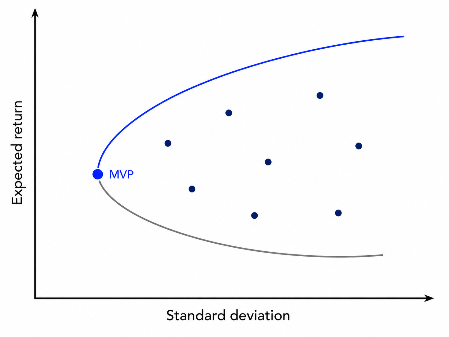
The MVP is the only portfolio on the efficient frontier that doesn’t require expected return estimates/forecasts

Finance theory makes the prediction that the market-cap weighted portfolio of securities is the optimal efficient portfolio in equilibrium, and should, in principle, outperform the MVP.

Although neat, this result is based on a list of strong assumptions, all of which are violated in practice. Therefore, even a comprehensive market-cap weighted portfolio of all stocks in the market is bound to be inefficient. This point was made by Haugen and Baker (1991), who compared such a portfolio (the Wilshire 5000) to an MVP constructed from the largest 1000 stock in the US, with some concentration and sector constraints. The MVP achieved similar returns to the market-cap weighted index, but with lower risk. de Silva, Clarke, and Thorley (2006) confirm this result with a long backtest, which shows that the MVP has about three-quarters of the realized risk of a cap-weighted portfolio, but earns higher average returns. Clarke, De Silva, and Thorley (2011) further study the composition of the MVP. They show that a long-only MVP typically invests in a small number of securities, tilted towards low betas.

The surprisingly good performance of the MVP relative to market-cap weighted portfolios is therefore related to the well-known critique of the CAPM (i.e., portfolios sorted on beta have negligible differences in return). More generally, this is related to the low beta and low volatility anomalies.

It should be noted that the MVP avoids expected return forecasts, but it still depends on a risk model (volatilities, correlations) and other choices like constraints and turnover assumptions.

The MVP is the only portfolio on the mean-variance efficient frontier that doesn’t require expected returns as inputs. In many long-run empirical studies, constrained minimum-variance portfolios have delivered lower volatility and competitive, sometimes higher, realized returns than capitalization-weighted indices.

An example of an investment product based on the MVP is the USMV ETF (about $24 billion in assets).

Alternative 3: Mean-Risk Optimization

As discussed above, the variance has some shortcomings as a risk measure. There are several alternative risk measures that can be used to replace the variance. The two most commonly used in practice are the semi-variance and the conditional Value at Risk (CVaR).

Mean-Semivariance Optimization

The semivariance is similar to the variance, but considers only returns below a benchmark level of return B:

$SV=\mathbb{E}\left[\left\{(R-B)\mathbb{1}_{r-b<0}\right\}^2\right]$

Intuitively, mean-semivariance optimization tries to find portfolios with attractive expected returns while penalizing only the observations in which the portfolio falls below the benchmark. This makes the relevant downside observations endogenous: changing the weights changes which scenarios count as downside scenarios.

For this reason, mean-semivariance optimization is not as simple as mean-variance optimization. The issue is that the semivariance of a portfolio cannot be written as a quadratic form, precluding the use of quadratic programming.

This problem can be resolved by noting that, within the regions where assets underperform the benchmark, the semivariance can be written in a quadratic form. This approach, presented by Markowitz et al. (2020), is the typical implementation used in practice. It relies on introducing a matrix of excess returns or deviations relative to the benchmark.

Mean-CVaR Optimization

To talk about conditional Value-at-Risk (CVaR), we first need to define the Value-at-Risk. Loosely speaking, the VaR is a loss that we’re fairly sure won’t be exceeded over some horizon. For example, suppose that the level of confidence is 90%. If the daily VaR of a portfolio with a 90% confidence level is $1 million, we are 90% confident that we won’t lose more than $1 million on any given day. Conversely, we should expect to lose more than $1 million on 10% of days.

VaR has some shortcomings as a way to measure risk. Notably, VaR is not a coherent risk measure. Particularly, VaR does not respect the sub-additivity property of a coherent risk measure, which requires that the risk measure applied to the sum of two portfolios must be at most equal to the sum of the risk measures applied to each portfolio. The consequence is that VaR may discourage diversification.

Another problem with VaR is that it only gives us a level of loss that we should not expect to exceed with some confidence, but it tells us nothing about what level of loss to expect when we do exceed it. The CVaR, or expected shortfall, gives you exactly that.

CVaR (also known as expected shortfall) is a tail risk measure. It tells us how much we expect to lose, given that the loss exceeds the VaR. The animation below shows examples of VaR and CVaR. Note that this is shown using the distribution of returns (i.e., negative values correspond to losses).

To define VaR and CVaR mathematically, we need some notation:

w : vector of portfolio weights
r : vector of asset returns
β ∈ (0,1) : confidence level
L(w, r) = -w’r: portfolio loss (negative of portfolio return)
p(r) : probability density function of returns
Ψ_L(y): cumulative distribution function of losses (the probability of not exceeding a threshold loss y).6
α_β(w): the VaR of portfolio w at confidence level β.

Note that we went from working with returns to working with losses. This means the distribution shown above would be flipped, with large positive values corresponding to large losses. With this notation, the VaR at confidence level β is defined as the smallest loss such that the probability of not exceeding it is at least β:

$\alpha_\beta(w)=\text{VaR}_\beta(w)=\min\{y\in \mathbb{R}:\Psi_L(y)>\beta\}$

Now that we have defined VaR, we can define the CVaR mathematically as:

$\text{CVaR}_\beta(w)=\frac{1}{1-\beta}\int_{L(w,r)\geq \alpha_\beta(w)}{L(w,r)p(r)dr}$

The expression above resembles the expected loss. Indeed, the CVaR_βis a specialization of the expected value in which we’re averaging only over the worst (1-β) fraction of losses.7

Portfolio optimization using the CVaR is complicated, because the CVaR depends on an integral over VaR values. However, Rockafellar and Uryasev (2000) proved two key results that make mean-CVaR optimization practical, effectively transforming it into a linear programming problem. Their paper rests on introducing the following function:

$F_\beta(w, \alpha)=\alpha+\frac{1}{1-\beta}\int_r{\left[L(w,r)-\alpha\right]^+p(r)dr}$

where[x]⁺=max(x,0). Their first theorem shows CVaR_β can be obtained as the minimum of this function in α. Their second theorem states that minimizingCVaR_β over all portfolios w is equivalent to minimizing the function above over all values of (w, α).

In practice, the integral can be approximated as a sum, using values that can be either simulated from p(r), if it’s available, or a sample (more commonly). Suppose that a sample of returns r₁, r₂, …, r_T is available. Then function can be approximated by

$F_\beta(w, \alpha)=\alpha+\frac{1}{(1-\beta)T}\sum_{t=1}^T{\left[-w'r_t-\alpha\right]^+}$

The optimization problem can then be written as a linear programming problem using auxiliary variables:

$\min_{w,\alpha}{\left\{\alpha+\frac{1}{(1-\beta)T}\sum_{t=1}^T{u_t}\right\}} \quad s.t. \left\{\begin{aligned} u_t&\geq 0\\ u_t&\geq -w' r_t-\alpha \end{aligned}\right.$

Mean-risk approaches replace variance with other risk measures. Two commonly used approaches are the mean-semivariance and mean-CVaR. Both optimization approaches are more complicated than MVO, but can be resolved by augmenting the optimization problem through auxiliary variables.

Alternative 4: Maximum Diversification

Choueifaty and Coignard (2008) note that one of the main difficulties with MVO is the need to estimate expected returns. They propose a heuristic approach based on maximizing the diversification ratio. Denote portfolio weights by w, the covariance matrix by Σ, and σ_d=diag(Σ)^1/2the vector of volatilities for the assets. The diversification ratio is defined as

$D(w)=\frac{w' \sigma_d}{\sqrt{w'\Sigma w}}$

The numerator is the weighted average of volatilities, which disregards diversification due to asset comovement. The denominator is the portfolio volatility, which accounts for asset comovement. Therefore, the diversification ratio captures the extent to which asset comovements reduce risk. They propose to compute the most diversified portfolio (MDP) by choosing w that maximizes this ratio. In their empirical applications, the MDP has higher Sharpe ratio than market-cap weighted indices.

MDP belongs to a class of risk-based portfolio construction approaches, which do not require estimation of expected returns. Other approaches in this category are the MVP and risk parity approaches.

A related paper is Clarke, De Silva, and Thorley (2013), who derive analytical expressions for risk-based portfolios (MVP, MDP, and risk parity) under a single-index model.

The maximum diversification approach selects portfolio weights that maximize the ratio between the weighted average volatility of the individual assets and the volatility of the resulting portfolio.

Alternative 5: Risk Parity

Risk parity is perhaps the most popular risk-based portfolio construction method. It is widely used by institutional investors because it provides a disciplined way to diversify risk. It is particularly popular with CTAs and trend followers to equalize how much risk each asset contributes to the overall portfolio.

A canonical example to explain risk parity is to look at a 60/40 portfolio of stocks and bonds. Using 10 years of data ending in April 2026, we get the following realized performance:

The 60/40 portfolio has a volatility of 11.3%. However, approximately 93.5% of this total risk comes from the equity allocation. The bond allocation, while representing 40% of the total allocation, accounts for less than 10% of the risk. Risk parity focuses on finding the portfolio allocations that would result in equal risk contributions. In this example, the allocations that equalize risk contributions are 23.6% in SPY and 76.4% in BND. The resulting portfolio has a volatility of 6.39%.

The example above uses volatility as the risk measure, but risk parity is more general. Denote by R(w) a risk measure for a portfolio w. The marginal risk contribution of asset i is defined as

$MRC_i= \frac{\partial R(w)}{\partial w_i}$

and the risk contribution of asset i is defined as

$RC_i=w_i MRC_i$

The risk measure must satisfy the Euler allocation principle, which states that risk can be decomposed as follows:

$R(w) =\sum_{i=1}^n{RC_i}= \sum_{i=1}^n{w_i MRC_i}$

In words: the total risk is the sum of the risk contributions, defined as each allocation multiplied by the derivative of the risk measure relative to the allocation. The portfolio risk can be obtained as the sum of risk contributions.

In the case of the volatility, we have

$\sigma=\sqrt{w'\Sigma w}$

and the vector of marginal risk contributions is

$MRC=\frac{\Sigma w}{\sqrt{w'\Sigma w}}$

Notice that the denominator is the same for all assets, such that the marginal risk contribution of asset i is:

$MRC_i=\frac{(\Sigma w)_i }{\sqrt{w'\Sigma w}}$

where (Σw)_i denotes the i-th element of Σw. We can verify that this satisfies the allocation property:

$\sum_{i=1}^n{RC_i}=\sum_{i=1}^n{w_i \frac{(\Sigma w)_i}{\sqrt{w'\Sigma w}}}=w'\frac{\Sigma w}{\sqrt{w'\Sigma w}}=\sqrt{w'\Sigma w}=\sigma$

Suppose that we have a risk budget b=(b₁, …, b_n) that defines how much risk each asset should contribute to the total risk. The risk parity case corresponds to equal risk contributions, i.e. b₁= ⋯ = b_n. The risk budget portfolio is the solution of the following system:

$\left\{ \begin{array} .RC_i&=b_i \\w_i&>0\\\sum_i{w_i}&=1 \end{array}\right.$

Writing the Lagrangian for this problem and solving the first-order conditions, it can be shown that it is equivalent to solving the following problem:

$\min_w \sigma(w) \quad s.t.\quad \left\{\begin{array}.\sum_{i=1}^n{b_i\ln{w_i}} \geq c \\w_i > 0, i=1,\dots, n\end{array}\right.$

One important element to consider when using the risk budget approach, especially with equal risk budgets, is that the choice of the asset universe can have a significant impact on the resulting portfolio. For instance, suppose we added another equity ETF to the universe in the toy example above. Then a risk parity solution would end up allocating 2/3 of the risk budget to equities and 1/3 to bonds. A possibility in these cases is to have equal risk budgets within asset classes, and divide asset-level risk budgets equally across instruments within each asset class.

A related approach is hierarchical risk parity. Rather than solving directly for equal risk contributions across all assets, hierarchical risk parity first uses the correlation structure to cluster similar assets, and then allocates risk through the resulting hierarchy. This can make the allocation less sensitive to small changes in the covariance matrix and can avoid some of the arbitrary effects of treating all assets in the universe as exchangeable.

There’s an enormous literature on risk parity and its performance. Some interesting earlier papers are Chaves, Hsu, and Thorley (2011), Asness, Frazzini, and Pedersen (2012), and Clarke, De Silva, and Thorley (2013). Hierarchical risk parity is introduced in Lopez de Prado (2016).

Note that risk parity is usually solved as a long-only problem with w_i > 0. In general, there’s no unique solution if weights are allowed to be negative. However, if we know which assets we want to short, a solution can be found by modifying the problem above. This approach is applied by Rubesam (2022) in the context of three systematic trading strategies (trend following, pairs trading, and factor investing).

Risk parity is a risk-based approach that constructs a portfolio so that assets or asset classes contribute equally, or according to predefined budgets, to total portfolio risk. Instead of allocating capital equally, it allocates risk equally.

Summary

Mean-variance optimization is often criticized due to the sensitivity of optimal solutions to changes in the inputs, estimation error, and due to the shortcomings of variance as a risk measure. At the same time, there are some persistent misconceptions about MVO, such as MVO requiring an assumption of normality or a quadratic utility function, which deserve to be put to rest.

This post reviews some alternatives to MVO, which range from doing away with forecasts altogether (1/N), getting rid only of expected return forecasts (MVP, MDP, risk parity), and using different risk measures (mean-semivariance, mean-CVaR). The table below summarizes these alternatives and their tradeoffs.

In an upcoming post, I’ll discuss a practical implementation of these alternatives with ETFs

I should not also that this is not an exhaustive list of alternatives to MVO. Another family of approaches, robust optimization, keeps the optimization framework but explicitly accounts for uncertainty in the inputs. Views-based approaches, such as Black-Litterman and Entropy Pooling, also remain close to the optimization tradition, but they change the way investor views, priors, or scenarios enter the problem. I will discuss these approaches in future posts.

References

Allen, D., Lizieri, C., & Satchell, S. (2019). In defense of portfolio optimization: What if we can forecast?. Financial Analysts Journal, 75(3), 20-38.

Asness, C. S., Frazzini, A., & Pedersen, L. H. (2012). Leverage aversion and risk parity. Financial Analysts Journal, 68(1), 47-59.

Benveniste, J., Kolm, P. N., & Ritter, G. (2024). Untangling universality and dispelling myths in mean-variance optimization. The Journal of Portfolio Management, 50(8), 90-116.

Chaves, D., Hsu, J., Li, F., & Shakernia, O. (2011). Risk parity portfolio vs. other asset allocation heuristic portfolios. Journal of Investing, 20(1), 108.

Choueifaty, Y., & Coignard, Y. (2008). Toward Maximum Diversification. The Journal of Portfolio Management, 35(1), 40-51.

Clarke, R., De Silva, H., & Thorley, S. (2011). Minimum-variance portfolio composition. Journal of Portfolio Management, 37(2), 31.

Clarke, R., De Silva, H., & Thorley, S. (2013). Risk parity, maximum diversification, and minimum variance: An analytic perspective. The Journal of Portfolio Management, 39(3), 39-53.

DeMiguel, V., Garlappi, L., & Uppal, R. (2009). Optimal versus naive diversification: How inefficient is the 1/N portfolio strategy?. The review of Financial studies, 22(5), 1915-1953.

De Silva, R., Clarke, H., & Thorley, S. (2006). Minimum-variance portfolios in the US equity market. Journal of Portfolio Management, 33(1), 1-14.

Dom, M. S., Howard, C., Jansen, M., & Lohre, H. (2025). Beyond GMV: the relevance of covariance matrix estimation for risk-based portfolio construction. Quantitative Finance, 25(3), 403-419.

Haugen, R. A., & Baker, N. L. (1991). The efficient market inefficiency of capitalization-weighted stock portfolios. Journal of Portfolio Management, 17(3), 35.

Jagannathan, R., & Ma, T. (2003). Risk reduction in large portfolios: A role for portfolio weight constraints. Journal of Finance, 58, 1651-1684.

Kritzman, M., Page, S., & Turkington, D. (2010). In defense of optimization: the fallacy of 1/N. Financial Analysts Journal, 66(2), 31-39.

Ledoit, O., & Wolf, M. (2003). Improved estimation of the covariance matrix of stock returns with an application to portfolio selection. Journal of Empirical Finance, 10(5), 603-621.

Lopez de Prado, M. (2016). Building diversified portfolios that outperform out-of-sample. Journal of Portfolio Management.

Markovitz, H. (1959). Portfolio selection: Efficient diversification of investments.

Markowitz, H. M., Starer, D., Fram, H., & Gerber, S. (2020). Avoiding the downside: A practical review of the critical line algorithm for mean–semivariance portfolio optimization. Handbook of Applied Investment Research, 369-415.

Pflug, G. C., Pichler, A., & Wozabal, D. (2012). The 1/N investment strategy is optimal under high model ambiguity. Journal of Banking & Finance, 36(2), 410-417.

Rockafellar, R. T., & Uryasev, S. (2000). Optimization of conditional value-at-risk. Journal of Risk, 2, 21-42.

Rubesam, A. (2022). The Long and the Short of Risk Parity. Journal of Portfolio Management, 48(4).

This approach has been pioneered in a series of papers by Ledoit and Wolf and their shrinkage estimators are widely available in portfolio optimization packages. These estimators can be helpful when the number of assets is large relative to the number of data points available. Dom et al. (2025) study the impact of the covariance matrix estimator for minimum variance portfolios. Sophisticated models do not add much value compared to the sample covariance matrix when long-only and turnover constraints are used.

Solving this problem for different levels of γ traces out the same efficient frontier as the more common approaches of minimizing the portfolio variance for different levels of expected return, or maximizing expected return for different levels of variance/volatility.

If we also assume decreasing absolute risk aversion, we can also make statements about investors’ preferences regarding skewness (investors prefer positive to negative skew) and kurtosis. If we also assume decreasing absolute prudence, investors dislike kurtosis.

Interestingly, this rule can even be optimal under extreme model uncertainty, as shown by Pflug et al. (2012).

Alternatively, it is the solution of mean-variance utility maximization stated previously with a coefficient of risk aversion γ→ ∞.

Note that we omit the dependence on the portfolio w.

That is,

$\text{CVaR}_\beta(w)=\mathbb{E}[L(w,r)|L(w,r)\geq \text{VaR}_\beta(w)]$

Systematically Biased

Discussion about this post

Ready for more?