
What Drives the Performance of Machine Learning Factor Strategies?
The use of ML in finance is all about the details

This week I’ll be heading to Braga in Portugal for the FMA European meeting, where I’ll be presenting a paper on forecast combination approaches for covariance matrix estimation. I will also be discussing the paper “What Drives the Performance of Machine Learning Factor Strategies”, by Mikheil Esakia and Felix Goltz, so I thought I’d share some points on this interesting paper.
A Common Setup for ML in Empirical Asset Pricing
A common setup in the literature on ML is the pooled or stacked regression approach, popularised in Gu, Kelly, and Xiu (2020, GKX). Suppose you have data on several firm characteristics (e.g.: size, book/market, momentum, etc) that past research has suggested are associated with expected returns. The idea is to build models of the form:
In words: we want to predict expected returns of stocks at time t+1, using predictors (typically stock characteristics) observed at time t, denoted by zi,t. The function g can be linear (e.g., ridge or lasso) or nonlinear (e.g., neural networks, random forests, boosted trees).
This approach is pooled because, each time you train the models, you effectively use information from all the stocks available. The characteristics in zi,t are typically cross-sectionally standardised, which helps with the scale and is also handy to imput missing values.1
GKX carried out an extensive horse race of linear and nonlinear models using U.S. data. They considered 94 firm characteristics from Green, Hand, and Zhang (2017, GHZ).2 The models in GKX included OLS, PLS, PCR, elastic net, generalized linear models, random forests, gradient boosted regression trees, and neural networks. The estimation setup in GKX uses expanding windows, starting with 18 years for training and 12 years for validation. Models are estimated once per year and used to forecast monthly returns for all stocks during that year. They then sorted stocks into decile portfolios based on next months forecasts.
GKX’s best performer in terms of statistical and economic performance was a neural network with 4 layers (NN4). The long-short portfolio constructed with NN4 forecasts yielded a Sharpe ratio of 1.35. GKX conclude that:
Neural networks and, to a lesser extent, regression trees, are the best performing methods. We track down the source of their predictive advantage to accommodation of nonlinear interactions that are missed by other methods.
That is, GKX attribute the superior performance of these methods to their ability to capture nonlinearities.
GKX was an important milestone in empirical asset pricing. It was among the first papers in the top finance journals to apply modern machine-learning methods at large scale to the cross-section of individual stock returns, with a careful out-of-sample design and a systematic comparison of methods. Its publication also signalled that ML had moved from being a largely peripheral or practitioner-oriented toolkit to something of broad interest within mainstream academic finance.
However, there are a number of caveats in that study:
Notably, GKX did not consider transaction costs. ML strategies generally have high turnover. For example, the NN4 long-short strategy had average monthly turnover of over 100% per month.
At any point in time, GKX used all the 94 characteristics from GHZ which had available data. This is a somewhat subtle form of look-ahead bias, as some of these characteristics were only identified with hindsight. As I discussed previously, we know from previous studies such as McLean and Pontiff (2016) that, once published, returns of characteristic-based anomalies diminish. Therefore, using the characteristics over the entire sample is likely to bias results upwards.
A Clever Design
Esakia and Goltz (2025, EG) implement a clever design aimed at disentangling the sources of return from ML factor strategies. The design is based on three pillars:
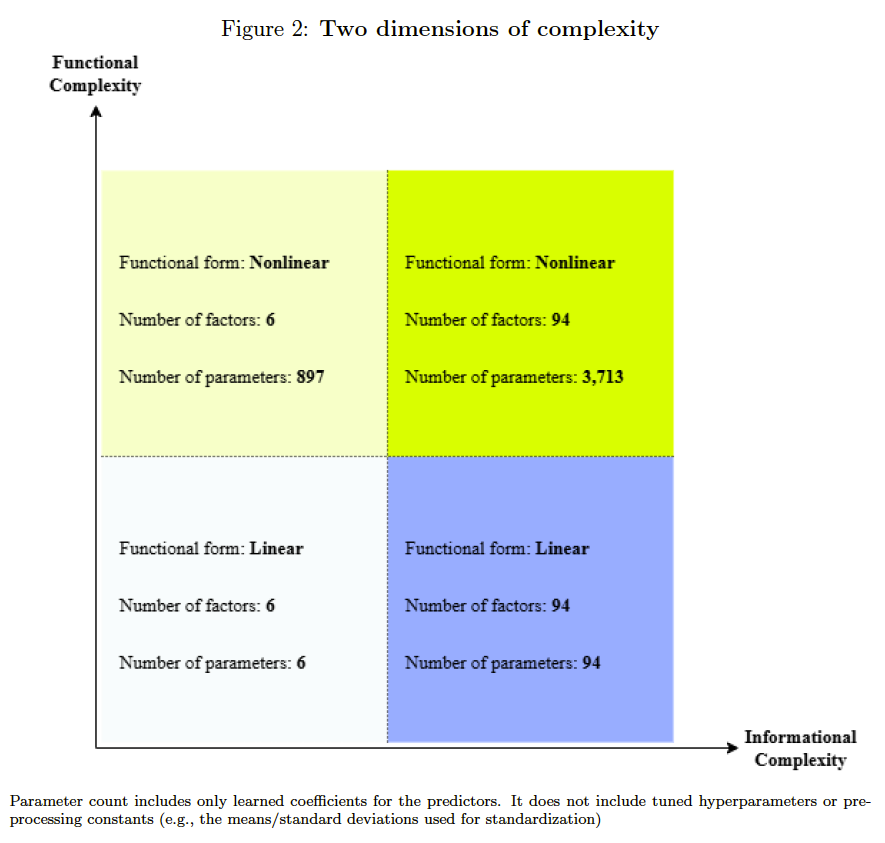
Assessing the value of different information sets and the flexibility of the functional form of the models;
Taking into account progressively more realistic implementation settings in terms of the universe of stocks used, factor hindsight, and transaction costs.
Starting with the information sets, EG consider two sets of characteristics:
The sparse set contains only “well known” factors such as beta, size, value, momentum, profitability, and asset growth.
The non-sparse set includes the full set of 94 characteristics.
The, in terms of flexibility, EG refrain from doing a horse race with many models. Instead, they consider the following representatives:
Linear model: ridge regression
Nonlinear model: a three-layer neural network
This gives the 2x2 design shown below:
In addition, EG consider different implementation settings, which are increasingly more realistic. These settings are summarized in their Table 1:
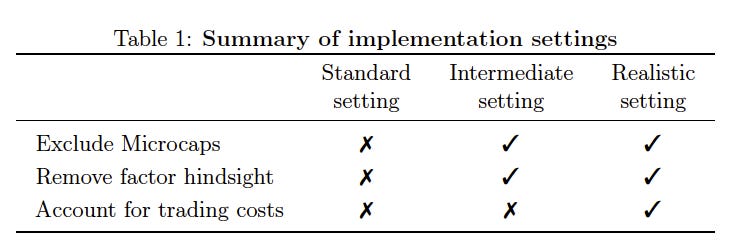
The Standard setting is similar to what is done in many papers. It does not explicitly exclude microcaps, and does not account for factor hindsight or trading costs. The Intermediate setting excludes microcaps and removes factor hindsight by only adding characteristic as they become publicly known. The Realistic setting also takes into account transaction costs. GKX’s paper sits between Standard and Intermediate, as they do tests some variations that exclude microcaps.
In terms of trading costs, EG first estimate effective bid-ask spreads using a method proposed by Chung and Zhang (2014), which only requires bid and ask quotes for each stock. Then, they implement an algorithm that assigns stocks to deciles based not only on expected returns, but looking at return differentials net of the cost of replacing a stock by another.
The Results
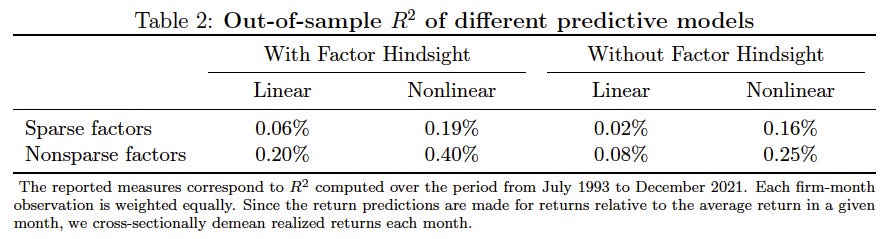
In terms of statistical performance, EG use the out-of-sample R2 as the metric. In line with other studies, their results confirm that the level of predictability in individual stocks is low. Their design shows that predictability deteriorates when removing factor hindsight, and improves when moving from linear to nonlinear models.
In terms of economic performance, however, the picture is very different. Their main results are shown below. The figure plots mean monthly returns under each implementation setting. As we move from the Standard to the Realistic setting, the mean return decreases significantly, as does the difference between linear and nonlinear. The decrease is economically very relevant: the performance of nonlinear models applied to the non-sparse set decreases from 3.63% per month in the Standard setting to 0.79% in the Realistic setting.
In the Standard setting, differences in mean returns suggest that both the information set and well as functional form complexity are statistically significant. In the Realistic setting, however, the difference is insignificant under the sparse set (i.e. from -0.07% to 0.14%) and only significant at the 10% level in the nonsparse set. The combined improvement in monthly returns of moving from linear models under the sparse set to nonlinear models under the nonsparse set is 0.86%, which is significant at the 1% level.

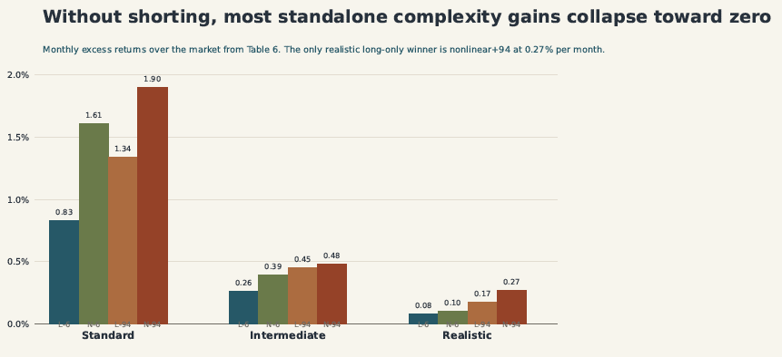
The paper also tests long-only versions of the strategies. Without allowing short positions, the gains from complexity shrink even more and become insignificant:
Final Thoughts
The main message of the paper is that, once you impose some realistic implementation assumptions, using a broader universe of firm characteristics is much more important than increasing the complexity of the functional forms used in the ML models. As ML becomes more widely used in finance, taking into account realistic implementation constraints is essential.
References
Chung, K. H. and H. Zhang (2014). “A simple approximation of intraday spreads using daily data”. Journal of Financial Markets 17, pp. 94–120.
Esakia, M., & Goltz, F. (2025). What Drives the Performance of Machine Learning Factor Strategies?. Available at SSRN 5851562.
Green, J., Hand, J. R., & Zhang, X. F. (2017). The characteristics that provide independent information about average US monthly stock returns. The Review of Financial Studies, 30(12), 4389-4436.
Gu, S., Kelly, B., & Xiu, D. (2020). Empirical asset pricing via machine learning. The Review of Financial Studies, 33(5), 2223-2273.
McLean, R. D., & Pontiff, J. (2016). Does academic research destroy stock return predictability?. The Journal of Finance, 71(1), 5-32.
Rubesam, A. (2022). Machine learning portfolios with equal risk contributions: Evidence from the Brazilian market. Emerging Markets Review, 51, 100891.
I used a similar approach in my 2022 paper looking at application of ML to the Brazilian equity market (Rubesam, 2022).
GHZ is another influential paper that looks into the factor zoo, but relies only on linear models. The authors made their SAS code available to download the firm characteristics data from CRSP/Compustat. This was before other initiatives like Open Source Asset Pricing existed.